How to Insert an In-Cell Picture in Microsoft Excel

Adding pictures to a Microsoft Excel worksheet can improve visualization, understanding, and overall presentation. However, floating images are notorious for causing layout issues when rows, columns, and cells are modified. To avoid these problems, you can embed pictures within cells.

Insert an In-Cell Picture Via the Excel Ribbon

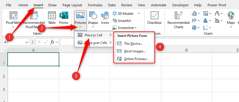
To insert an in-cell picture saved on your device, from Microsoft’s gallery, or imported through the web images search, first, select a blank cell. Then, in the Insert tab on the ribbon, click “Pictures,” hover over “Place In Cell,” and select one of the options.

When you select the picture and click “Insert,” you’ll see it embedded within the active cell.

In-cell images inserted in this way adapt to the cell size while maintaining their aspect ratio, so click and drag the boundaries between the column and row headers to resize them.

When you select the cell containing the in-cell image, you’ll see the word Picture in the formula bar.

That said, if you add alt text to the in-cell picture by right-clicking the cell and selecting “View Alt Text,” you see this in the formula bar instead.

The usual cell formatting can be applied to cells containing in-cell pictures. For example, you can center the image by clicking the “Center” icon in the Alignment group or fill the cell with a certain color by clicking the “Fill Color” down arrow in the Font group.

Paste a Picture You Just Copied Into a Cell in Excel

You can insert a picture into a cell in Microsoft Excel by copying and pasting it. The image could be copied from another Excel workbook, a Word document, an email, an online source, or—in fact—anywhere, provided it’s a format supported by Excel and you have permission to use it.

If the picture you want to insert in-cell is the last thing you copied, head to the cell where you want it to appear. Then, in the Home tab on the ribbon, click the “Paste” down arrow, and select the icon which looks like a clipboard with a picture over the top.

Alternatively, if you prefer using Excel keyboard shortcuts, press Alt > H > V > C.

As with in-cell pictures added via the Insert tab on the ribbon, pasted in-cell pictures grow and shrink when the cells they’re in change size, but their aspect ratio remains the same. Also, when the cell containing the in-cell picture is selected, you’ll see the word Picture in the formula bar, unless you add alt text.

Insert an In-Cell Picture Using Excel’s IMAGE Function

In-cell pictures can be inserted into an Excel spreadsheet through the IMAGE function. Use this method if you’ve found a picture on the web that you want to insert into a cell, provided you have permission to do so.

Here’s the IMAGE function’s syntax:

=IMAGE(a,b,c,d,e)

The five arguments work as follows:

When using the IMAGE function, bear in mind the following points:

• Images with URLs requiring authentication cannot be inserted into a cell, and URLs that redirect to another address are blocked.
• URLs (and all other text values) in formulas are limited to 255 characters. If the image URL contains 256 or more characters, paste it into another cell, and reference this cell for argument a.
• Excel returns the #VALUE! error if the image file isn’t in a supported format, or you forget to wrap the URL or alt text inside quotation marks.
• If you enter 3 for argument c, but don’t specify an image height (argument d) or width (argument e), the formula won’t work. You’ll also face similar problems if you enter values for arguments d or e without entering 3 for argument c.
• If you see the #CONNECT! error, check your internet connection and try again.

To try this out, triple-click the following URL (a picture containing the How-To Geek logo from the Valnet website) to select it, and press Ctrl+C to copy it:

https://www.valnetinc.com/images/brand-backgrounds/htg-bg2.jpg

Now, open a new workbook, and in cell A1, type:

=IMAGE("

Then, press Ctrl+V to paste the copied URL. At this point, you’ll see a security alert asking you to confirm whether you want to paste the image URL with or without active content. Click “Paste Without Active Content.”

Next, add closing quotation marks and a comma, and for argument b (the alt text), type:

"The How-To Geek logo."

Finally, close the parentheses, and press Enter.

Because you haven’t specified the picture’s dimensions, it fits inside the cell, growing and shrinking as you alter the cell’s dimensions.

However, suppose you decide you want to fix the picture’s height to 200px. To do this, head back to cell A1, and press F2 to activate Edit mode. Then, use the Arrow keys to move the cursor inside the closing parenthesis, and add a comma. Then, for argument c, type 3, and add another comma.

Finally, for argument d (image height), type 200, and press Enter to commit the new formula.

The picture is now 200px high, and the original aspect ratio is preserved because you didn’t type a width dimension for argument e. This means the cell may need to be resized to make the whole picture visible.

Convert a Floating Picture Into an In-Cell Picture in Excel

If your Excel worksheet already contains a picture placed over the cells, you can turn this into an in-cell picture in no time.

First, click and drag the image so that the top-left corner is over the cell where you want the in-cell image to be. In this example, I want the How-To Geek logo to be inserted into cell B2.

Next, click the “Place In Cell” icon that appears directly next to the picture when it’s selected.

Alternatively, right-click the floating picture, and click “Place In Cell.”

Floating pictures converted into in-cell pictures adapt to changes in the cell size while retaining their aspect ratio.

Format In-Cell Pictures in Excel

Pictures inserted on top of cells can be formatted via the Picture Format tab on the ribbon. However, as you can see in the screenshot below, when a cell containing an in-cell picture is selected, the Picture Format tab doesn’t appear.

So, to format an in-cell picture in Excel, you need to temporarily turn it into a floating image. To do this, right-click the cell containing the picture, hover over “Picture In Cell,” and click “Place Over Cells.”

Alternatively, for in-cell images that have been pasted or inserted via the ribbon, a quicker method is to select the cell, and click the “Place Over Cells” icon that appears.

Now, you can format the picture using the tools in the Picture Format tab on the ribbon.

Once you’ve finished formatting the picture, convert it back into an in-cell picture by right-clicking the image and selecting “Place In Cell,” or clicking the “Place In Cell” icon that appears when you select the picture.

Pictures serve many purposes in Excel worksheets aside from forming the content of a cell. Indeed, you can use images as chart columns, insert dynamic pictures in a dashboard, or create worksheet thumbnails in a visual table of contents.

OS

Windows, macOS, iPhone, iPad, Android

Free trial

1 month

Microsoft 365 includes access to Office apps like Word, Excel, and PowerPoint on up to five devices, 1 TB of OneDrive storage, and more.