IPython and Jupyter aren’t IDEs—and that’s exactly why I use them for data science

Lots of people will use an IDE like VS Code or a regular editor like Vim, but for my work in data science and statistics, I need something different. Here’s why I use IPython and Jupyter notebooks for exploring datasets.

Exploratory programming

IPython and Jupyter let you explore data

IPython and Jupyter offer something different than the standard scripting or IDE workflow. They’re interactive programming tools. You can type in some code and see instantly what will happen. You don’t have to write a script or program and run it.

This opens the door to a new style of development. Instead of having a goal in mind, you can try different approaches. One reason that statistics and data science have taken up notebooks is that these disciplines are suited to the exploratory style that IPython and Jupyter encourage. If you’re examining a dataset, you’ll probably not have an idea of what it contains. Once you can summarize it and graph it, what you can do with it becomes much clearer.

IPython

A better interactive Python interpreter

While the standard Python interpreter is helpful for testing out ideas and learning the language, if you try to make heavy use of it, you run into its limitations. One big thing missing from the standard Python interpreter is tab completion. It’s also difficult to re-run code you’ve already run.

IPython is a big help. It includes tab completion. You just hit the Tab key and IPython will fill in things like functions or variable names. You can also zip back and forth in your history, and search your previously typed commands. It works the same way as modern Linux shells do, using the GNU Readline library.

Another handy feature is built-in “magic” commands. These are prefaced with a percent sign (%). One useful magic command is the “timeit” command.

I’ll demonstrate by first generating a 10 x 3 array in NumPy, which will be X, and a randomly generated array of 10 numbers, which I’ll designate y.

import numpy as np

rng = np.random.default_rng()

X = rng.random((10,3))

y = rng.random(10)

Then I’ll compute the least-squares solution and time it:

%timeit np.linalg.lstsq(X,y)

The time it took to execute will be returned:

In this case, it took about 12 microseconds, which is pretty fast, though this is a small matrix. A bigger one might take longer:

X = rng.random((500,3))
y = rng.random(500)

%timeit np.linalg.lstsq(X,y)

The result is approximately 22 microseconds. This is still fast for a large linear system.

Jupyter

Mix text, code, and graphics

While IPython is a great interactive terminal program for Python, Jupyter takes it to the next level. Jupyter is an interactive notebook program. Jupyter lets you mix code, text, and inline plots. It’s a form of “literate programming,” a term coined by legendary computer scientist Donald Knuth.

Jupyter notebooks are similar to the notebook interfaces in programs like Mathematica. A notebook is built out of cells that can contain code or Markdown text. While Jupyter was originally an offshoot of IPython, it also allows you to use other programming languages like R, Julia, or Scala.

Here’s a screencast by Rob Mulla demonstrating how to create a Jupyter notebook:

The best feature of a Jupyter notebook is its persistence. I can explore a dataset with Python, and when I come back to it, I can remember what I did.

When would I use either

Exploration vs. persistence

There are some clear use cases for both IPython and Jupyter. For quick experimentation, I’ll turn to IPython. I’ll often leave it running in a background terminal. I’ve created a Pixi environment with NumPy, SymPy, and other mathematical Python libraries to give me the ultimate desk calculator.

While IPython is handy for quick calculations and throwaway computations that I’m likely not going to need to refer to later, Jupyter is useful for data exploration that I’m going to want to come back to or share with others. I’ve already uploaded a handful of my own statistical explorations in Jupyter notebooks to my GitHub account.;

Vim is still my editor of choice for regular scripts and tweaking configuration files.

A typical stats workflow

Putting it all together

I’ll demonstrate briefly by opening up a Jupyter notebook. I’ve already installed Jupyter in a directory called “stats.” An environment in Pixi is simply a directory. I want to demonstrate this in a reproducible environment. I’ve uploaded my notebook to my GitHub repository.

I’ll start up the Jupyter server:

jupyter notebook

I’ll create a new notebook. I’m going to examine a predefined data set of data taken by a waiter in a New York City restaurant, who recorded the total bill, the tip, the number of diners in the party, and whether any of them were smokers.

I’ll create a cell that includes the libraries I want to use:

import numpy as np
import pandas as pd
import seaborn as sns
sns.set_theme()
from scipy import stats
import statsmodels.api as sm
import statsmodels.formula.api as smf
%matplotlib inline

This imports NumPy, pandas, Seaborn, the stats submodule from SciPy, statsmodels, and its formula API, and tells matplotlib to insert any plots into the Jupyter notebook instead of opening them in a separate window.

With the libraries imported, I can load the tips database from Seaborn, which has some built-in datasets mainly for plotting. This will be stored as a pandas DataFrame.

tips = sns.load_dataset('tips')

I’ll look at the top of the dataset.

tips.head()

Then I’ll take descriptive stats of the numerical columns. This includes the mean, the standard deviation, the minimum, the lower quartile (25th percentile), the middle value or median, and the upper quartile (75th percentile).

tips.describe()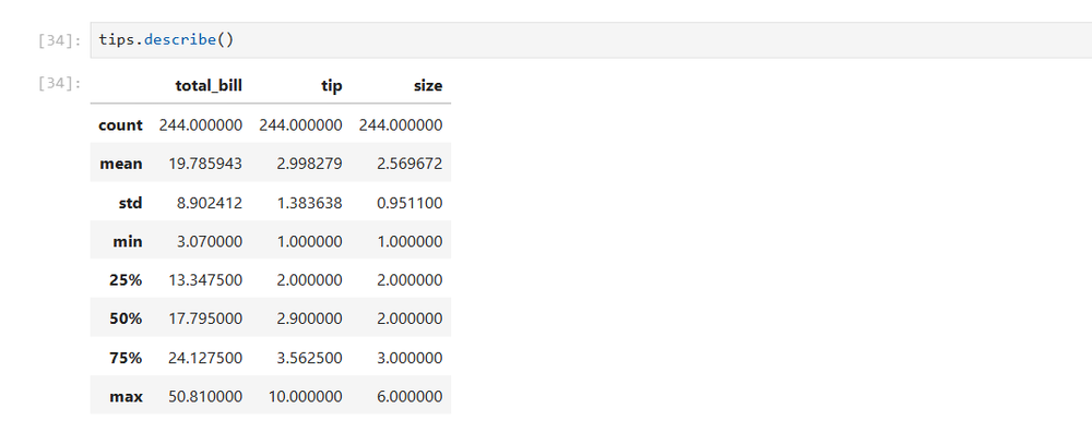

Next, I want to look at the distribution of the total bill:

sns.displot(x='total_bill',data=tips)

And the tips:

sns.displot(x='total_bill',data=tips)

Now I’ll look at the scatterplot of tip vs bill:

sns.relplot(x='total_bill',y='tip',data=tips)

I can plot a regression line over the scatterplot:

sns.regplot(x='total_bill',y='tip',data=tips)

There seems to be a positive linear relationship, since the line slopes upward. I’ll need to use statsmodels to get the values to plug into the classic equation y = mx + b using a formula notation popularized by R.

results = smf.ols('tip ~ total_bill',data=tips).fit()
results.summary()

The values for the y-intercept and the slope (m), in this case, the total bill, are listed in the left-most column in the table.

Building a program bottom-up

The best thing about interactive programming is that you can start with nothing and end up with a complete analysis. It’s a kind of bottom-up programming where you build a program through exploration, and then you can share your results with others.